LIBS-System: First test-run

The new system is faster, easier to use, and works with a higher resolution. See the EGU conference presentation here or below under Related

Niklas

Last updated on Mar 22, 2022 3 min read

Project

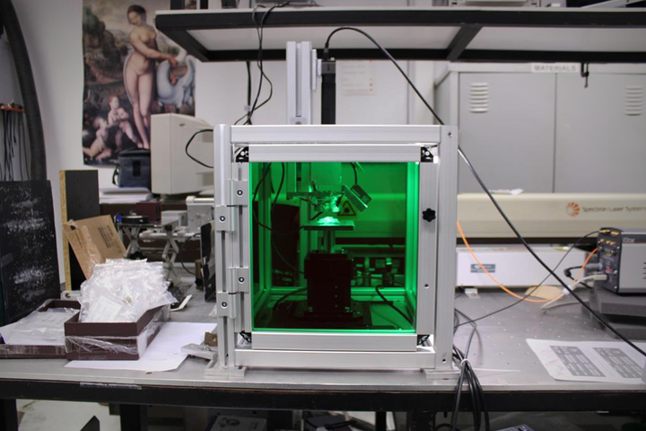
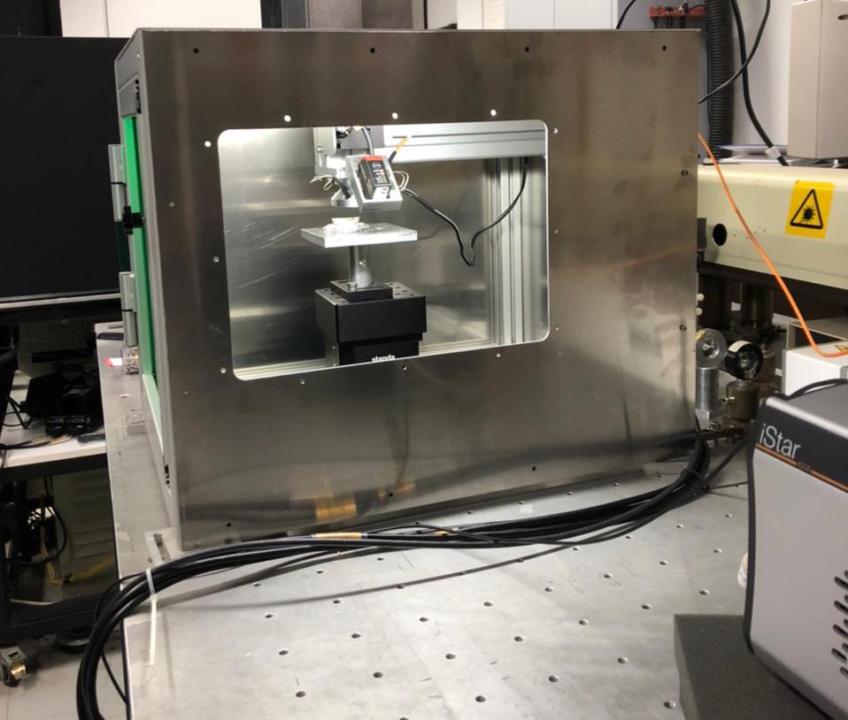
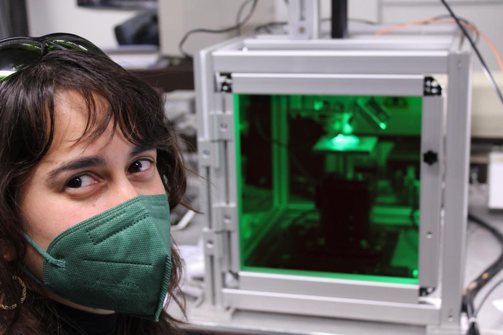
After only communicating via email and videoconferences for almost a year and a half, the project members finally met up for an in person meeting on Crete to test and discuss the new LIBS-system. Victor Piñon and Andreas Lemonis at FORTH have been busily putting together our hardware components over the last few months and turned them into a working machine.

*Side view of the system with protective glass not inserted yet.*

New equipment and resolutions

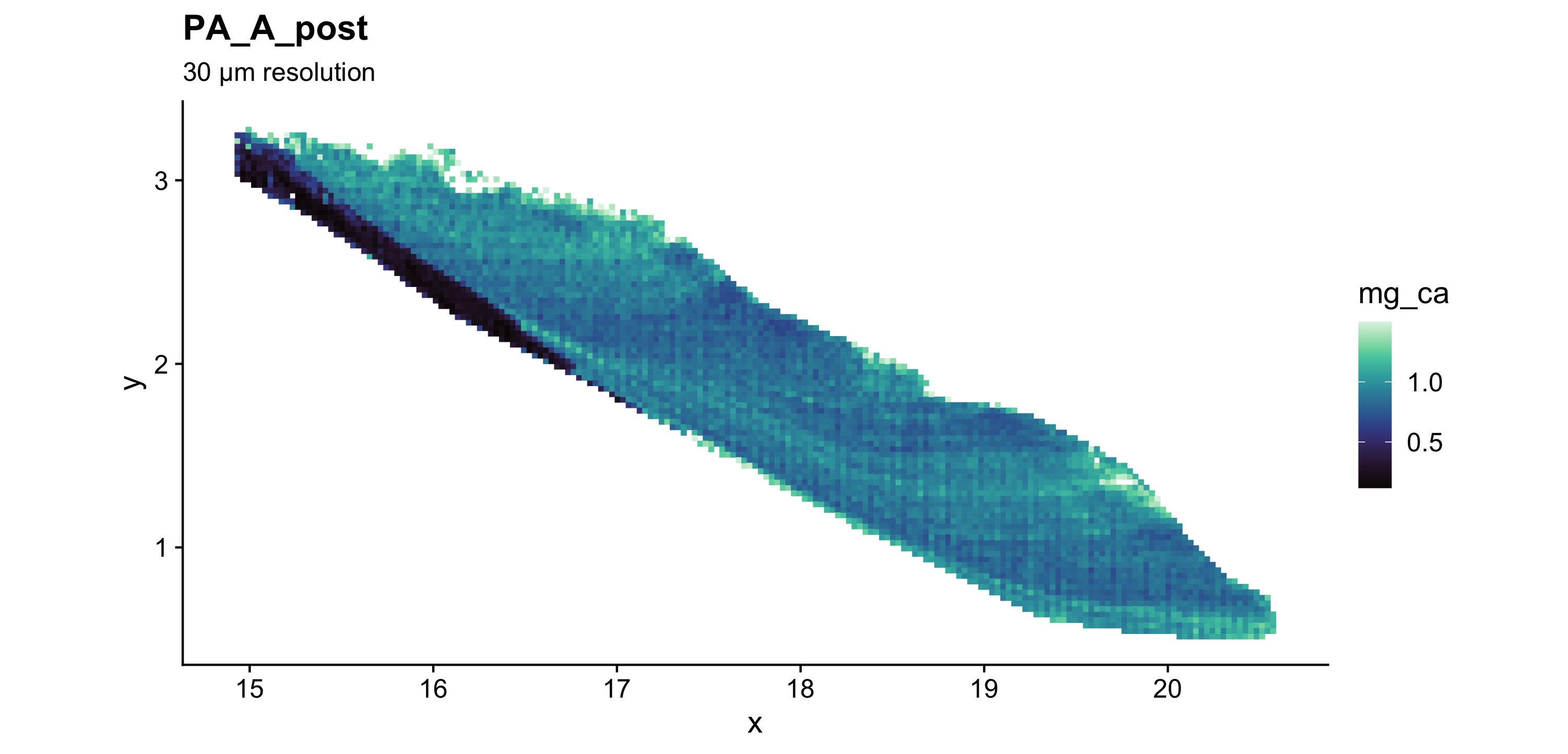
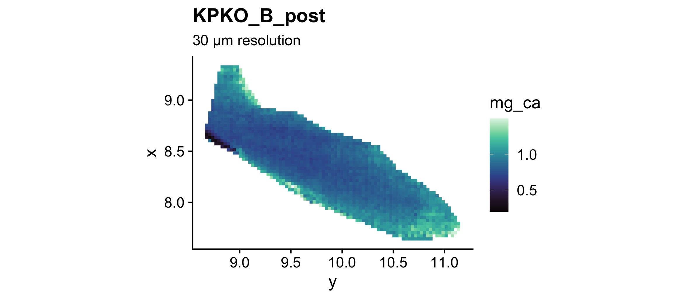
It is a great step forward from our previous system, with a faster laser (100 Hz rather than 10 Hz) and a more accurate optical apparatus that works on a lower energy (1.5 mJ rather than 15 mJ), which makes the analysis faster and less destructive than before. We are still in the progress of getting accurate measurements of the dimensions of each sampling spot, but it looks like we moved from 50 µm down to 30 µm with the potential to go even lower, using single shot measurements. Maybe it will be enough to measure daily increments (5–10 µm) on our limpet shells?

*Danai using the new LIBS-system. No glasses needed with the protective front window!*

The testing material has been sourced from all over Greece, where Danai has been collecting live limpet shells near archaeological sites (e.g. Franchthi, Agios Petros and Cyclop’s cave). These limpets will be the foundation for the sclerochronological analysis of our modern reference to understand the data coming from the archaeological samples.

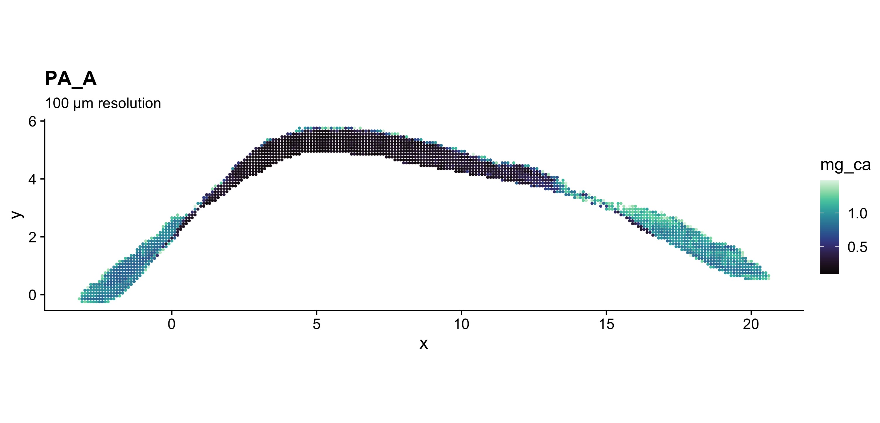
Elemental mapping will be the first step to understand the shell’s growth structure and carry out a more targeted analysis of δ¹⁸O values later on, saving us time and money (and nerves).

The LIBS-system has a new user-friendly interface so that we can more easily describe the sampling area that we want to map. Shells can have quite complex sections, so a good control of where exactly the data comes from is very important.

*Outlining the shell has become much easier by simply pointing and clicking.*

Once the outline is defined, we interpolate the area with sample spots at ~30 µm distance. With the new 100 Hz laser we can sample up to 13 spots those per second, depending on how many spectra we choose for each location (e.g. 10 spectra/spot allows us to sample ~6 spots per second). So that even a map of 2000 points ( which used to take an hour) will only take just over 5 minutes.

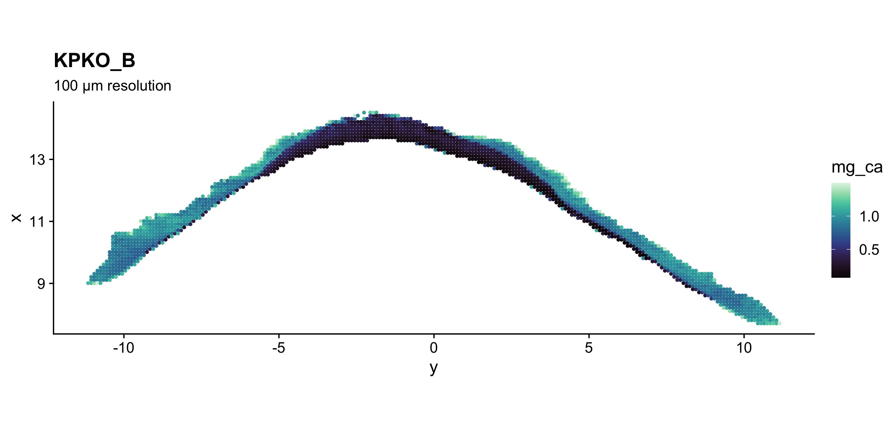
*Live sampling doesn’t always show the plasma if the framerate is in sync but you can see the craters on the video and the plasma on the sample.*

Here are some of the examples that we ran over the last few weeks. We are still working on the data-visualisation component. The maps below have been made with R and ggplot:

*This shell is from Alonnisos and was collected close to the end of Summer. Its scan took about 5 minutes for 19 mm ².*

The summer signal (high Mg/Ca) on the edge is better visible in this high resolution scan. The scan took about 13 minutes, because of its higher resolution (30 µm), although it is a smaller area (~4.6 mm²).

*This shell is from Kyra Panagia and was also collected close to the end of Summer. This scan took about 5 minutes for 17 mm².*

As above, the summer signal (high Mg/Ca) on the edge is better visible in the high resolution scan. This scan took about 5 minutes, as we had a higher resolution but scanned a much smaller area (~1.5 mm²).

LIBS SEAFRONT